Climate change and temperature anomalies

If we wanted to study climate change, we can find data on the Combined Land-Surface Air and Sea-Surface Water Temperature Anomalies in the Northern Hemisphere at NASA’s Goddard Institute for Space Studies. The tabular data of temperature anomalies can be found here

To define temperature anomalies we need to have a reference, or base, period which NASA clearly states that it is the period between 1951-1980.

weather <- 
  read_csv("https://data.giss.nasa.gov/gistemp/tabledata_v4/NH.Ts+dSST.csv", 
           skip = 1, 
           na = "***",
           show_col_types = FALSE)

tidyweather <- weather %>%
  select(1:13) %>%
  pivot_longer(
    cols=2:13,
    names_to = 'Month',
    values_to = 'delta'
  )

Plotting Information

Let us plot the data using a time-series scatter plot, and add a trendline. To do that, we first need to create a new variable called date in order to ensure that the delta values are plot chronologically.

tidyweather <- tidyweather %>%
  mutate(date = ymd(paste(as.character(Year), Month, "1")),
         month = month(date, label=TRUE),
         year = year(date))

ggplot(tidyweather, aes(x=date, y = delta))+
  geom_point()+
  geom_smooth(color="red") +
  theme_bw() +
  labs (
    title = "Weather Anomalies"
  )

## `geom_smooth()` using method = 'gam' and formula 'y ~ s(x, bs = "cs")'

## Warning: Removed 4 rows containing non-finite values (stat_smooth).

## Warning: Removed 4 rows containing missing values (geom_point).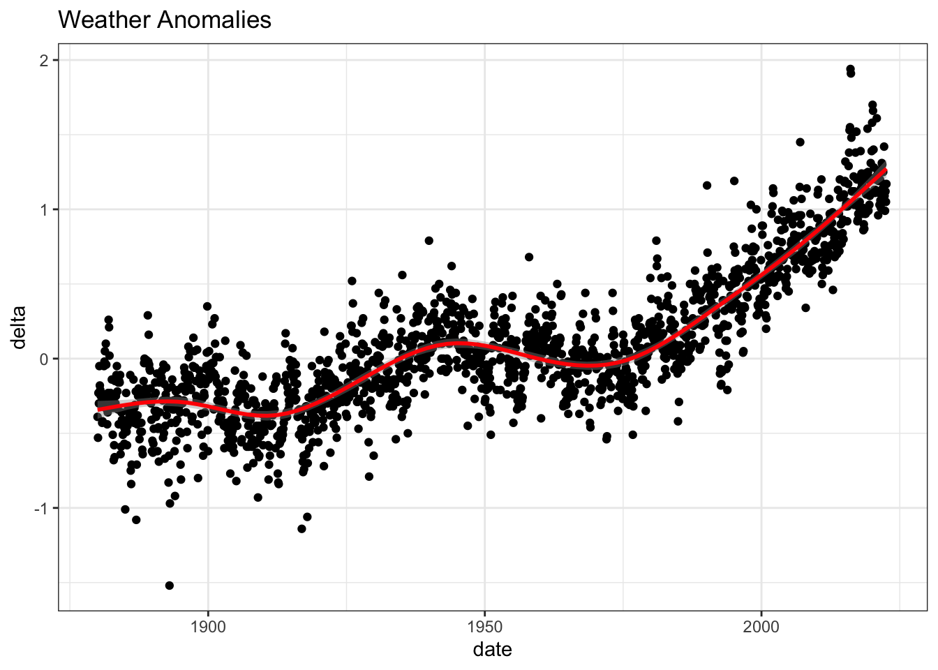

Producing a seperate scatter plot for each month, again with a smoothing line.

## `geom_smooth()` using method = 'loess' and formula 'y ~ x'

## Warning: Removed 4 rows containing non-finite values (stat_smooth).

## Warning: Removed 4 rows containing missing values (geom_point).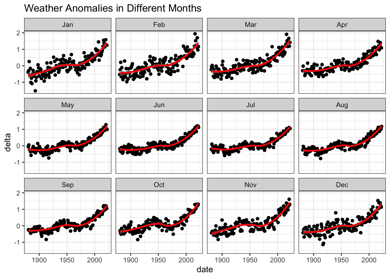

It is sometimes useful to group data into different time periods to study historical data. For example, we often refer to decades such as 1970s, 1980s, 1990s etc. to refer to a period of time. NASA calcuialtes a temperature anomaly, as difference form the base periof of 1951-1980. The code below creates a new data frame called comparison that groups data in five time periods: 1881-1920, 1921-1950, 1951-1980, 1981-2010 and 2011-present.

We remove data before 1800 and before using filter. Then, we use the mutate function to create a new variable interval which contains information on which period each observation belongs to. We can assign the different periods using case_when().

comparison <- tidyweather %>% 
  filter(Year>= 1881) %>%     #remove years prior to 1881
  #create new variable 'interval', and assign values based on criteria below:
  mutate(interval = case_when(
    Year %in% c(1881:1920) ~ "1881-1920",
    Year %in% c(1921:1950) ~ "1921-1950",
    Year %in% c(1951:1980) ~ "1951-1980",
    Year %in% c(1981:2010) ~ "1981-2010",
    TRUE ~ "2011-present"
  ))

Now that we have the interval variable, we can create a density plot to study the distribution of monthly deviations (delta), grouped by the different time periods we are interested in. Set fill to interval to group and colour the data by different time periods.

ggplot(comparison, aes(x=delta, fill=interval))+
  geom_density(alpha=.3)

## Warning: Removed 4 rows containing non-finite values (stat_density).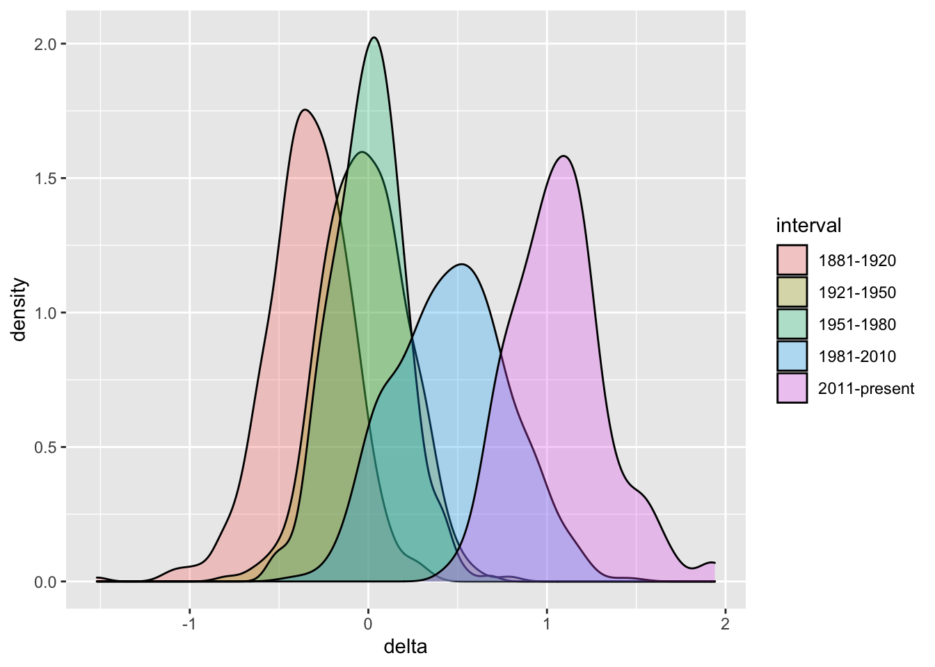

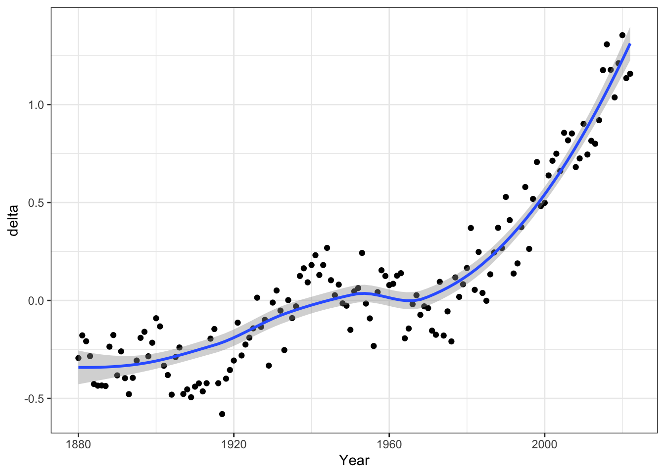
So far, we have been working with monthly anomalies. However, we might be interested in average annual anomalies. We can do this by using group_by() and summarise(), followed by a scatter plot to display the result.

#creating yearly averages
average_annual_anomaly <- tidyweather %>% 
  group_by(Year) %>%   #grouping data by Year
  
  # creating summaries for mean delta 
  # use `na.rm=TRUE` to eliminate NA (not available) values 
  summarise(delta = mean(delta, na.rm=TRUE)) 

#plotting the data:

ggplot(average_annual_anomaly,aes(x=Year,y=delta))+
  geom_point()+
  geom_smooth(method = "loess")+
  theme_bw()

## `geom_smooth()` using formula 'y ~ x'